Adapting a 2026 speech recognizer for English, Hindi, Singlish and Hinglish
In this article
- The 2026 candidate
- Define the transcript convention first
- Build four data slices
- Keep a manifest that can explain every example
- Hardware and memory
- An executable-shaped training recipe
- Streaming the model
- What the completed public Whisper experiment actually found
- The release decision for the new model
- The data review that should happen before the first GPU hour
- Know which tokens receive loss
- Separate adaptation from decoding and runtime changes
- A streaming test must not see the future
Fine-tuning becomes useful when the recognizer's errors have a pattern: recurring vocabulary, a particular accent, code-switching, or the acoustic conditions of the telephone channel. It is much less useful when the underlying problem is incorrect sample-rate handling or an inconsistent transcript convention.
We fine-tuned Whisper in late 2024. In September 2026, I revisited the problem with a public-data Whisper Tiny experiment whose training and evaluation results are included below. I then use Qwen3-ASR to work through the next adaptation recipe for English, Hindi, Singlish and Hinglish.
The Tiny results are the completed experiment. The Qwen sections give you the model, data, training and serving configuration for the next comparison.
The 2026 candidate
Qwen3-ASR was released in January 2026 in 0.6B and 1.7B variants. Its published language coverage includes English and Hindi. The smaller model is the initial candidate because the problem is interactive serving with a limited hardware budget, not maximizing an offline leaderboard score. Qwen3-ASR technical report, 0.6B model card.
Singlish and Hinglish remain evaluation targets, not capabilities established by that language list. Tamil and Telugu require a separate candidate or an existing provider path; they are not in this model's published ASR language list.
The upstream repository includes fine-tuning support and a streaming interface. At the inspected revision, streaming is available through the vLLM backend, and the documented streaming interface does not support batched inference or timestamps. Offline batching should not be advertised as evidence of equivalent streaming concurrency. Qwen3-ASR repository.
Define the transcript convention first
Consider this constructed example:
Audio meaning: मुझे policy renew नहीं करनी।
Mixed-script reference: मुझे policy renew नहीं करनी
Romanized reference: mujhe policy renew nahi karni
Meaning-changing error: मुझे policy renew करनी
The first two references can describe the same speech. The last line loses the negation.
Primary evaluation should use a declared script and normalization policy. A secondary transliteration-tolerant score can expose script differences, but should not replace the raw record or conceal semantic errors. Track negations, amounts, dates, policy IDs and names separately.
For Singlish, do not automatically normalize every local expression into formal English. That can erase the phenomenon the experiment is intended to recognize. Retain the spoken form in the primary transcript and use a separate downstream normalization layer if the business workflow requires it.
Build four data slices
The proposed first adaptation set is deliberately modest: 40 hours, allocated as 10 hours each of ordinary English, Hindi, Singapore English/Singlish and Hindi–English code-switching. These are collection targets, not data already assembled.
| Slice | Candidate source | Important limitation |
|---|---|---|
| Hinglish | MUCS Hindi–English, OpenSLR 104 | Technical tutorials differ from customer calls |
| Singapore English | IMDA National Speech Corpus | Select suitable conversational material and verify access/terms |
| Hindi | Audited native-speaker recordings or a licensed public corpus | Avoid treating synthetic speech as the entire test |
| General English | Licensed recordings covering intended accents | Preserve an ordinary-English regression set |
OpenSLR 104 describes 89.86 training hours and 5.18 test hours of Hindi–English speech, sampled at 16 kHz, with code-switching largely arising from technical tutorial content. That makes it a useful public illustration, not a substitute for telephone-domain evidence. OpenSLR 104.
IMDA describes NSC as a Singapore English audio/transcript corpus. Its relevance is local speech coverage; it is not a turnkey claim that every Singlish use case is represented. IMDA National Speech Corpus.
Split by speaker and source recording before segmentation. Keep duplicate and near-duplicate audio out of validation and test. Reserve a separate real telephone test with new speakers; telephone simulation applied to tutorial audio remains simulation.
Keep a manifest that can explain every example
{
  "sample_id": "illustrative-hi-en-0001",
  "audio": "audio/illustrative-hi-en-0001.wav",
  "text": "मुझे policy renew नहीं करनी",
  "slice": "hinglish",
  "speaker_group": "speaker-017",
  "session_group": "session-004",
  "source_group": "recording-004",
  "sample_rate": 16000,
  "duration_seconds": 3.8,
  "source_revision": "resolve-before-training",
  "split": "train",
  "augmentation": "none"
}
This is a schema example, not an existing recording.
The training export converts the manifest to the upstream trainer's audio/text format. Preserve the richer manifest for audit and evaluation. For code-switched data, test the supported language-prefix convention on development data rather than inventing a new “Hinglish” special token.
Hardware and memory
A proposed starting machine for the 0.6B experiment is one NVIDIA L4 or A10G with 24 GB VRAM, at least 32 GB host RAM and 100 GB free local storage. Begin with microbatch one and short clips. This is an engineering estimate, not a measured minimum.
At 600 million parameters, BF16 weights alone occupy roughly 1.2 GB in decimal units. Full training also needs gradients, optimizer state, activations, temporary buffers and sometimes master weights. A rough 16-bytes-per-parameter accounting reaches 9.6 GB before activations. The exact implementation can differ, so observe allocated and reserved memory during a real forward/backward pass.
If the required sequence length does not fit, first reduce the microbatch and audit padding. Then use a training configuration that explicitly supports activation checkpointing, or move to a 48 GB GPU. Do not claim the upstream trainer supports LoRA or checkpointing flags without implementing and verifying them.
An executable-shaped training recipe
The upstream trainer accepts JSONL audio/text pairs. Start with the configuration below, and pin the upstream commit, model revision and environment so that a result can be reproduced. Qwen fine-tuning guide, trainer implementation.
python finetuning/qwen3_asr_sft.py \
  --model_path Qwen/Qwen3-ASR-0.6B \
  --train_file data/train-qwen.jsonl \
  --eval_file data/dev-qwen.jsonl \
  --output_dir artifacts/qwen3-asr-adapted \
  --batch_size 1 \
  --grad_acc 16 \
  --lr 1e-5 \
  --epochs 2 \
  --warmup_ratio 0.05 \
  --save_steps 100 \
  --save_total_limit 4 \
  --num_workers 2
This specifies full-model adaptation, effective batch 16 on one GPU, and a conservative initial learning rate. It is a starting point rather than an optimum.
Training loss is not the release metric. Decode a frozen development set at selected checkpoints and compute corpus WER plus entity errors by slice. The upstream evaluation path should not be assumed to select checkpoints on decoded WER merely because an evaluation file is supplied.
Use development results to select checkpoint and decoding settings. Run the final test once after selection. If the result inspires another round of tuning, preserve it and use a new experimental record.
Streaming the model
The official streaming example exposes state initialization, incremental transcription and a final flush. A minimal adapted API illustration is:
from qwen_asr import Qwen3ASRModel

def transcribe_stream(chunks_16k):
    model = Qwen3ASRModel.LLM(
        model="Qwen/Qwen3-ASR-0.6B",
        gpu_memory_utilization=0.70,
        max_new_tokens=32,
    )
    state = model.init_streaming_state(
        unfixed_chunk_num=2,
        unfixed_token_num=5,
        chunk_size_sec=2.0,
    )
    for chunk in chunks_16k:
        model.streaming_transcribe(chunk, state)
        yield state.text
    model.finish_streaming_transcribe(state)
    yield state.text
This illustrates API shape using mono float audio at 16 kHz; it is not a network server. Model initialization belongs at worker startup in production, not once per call. Results are revised cumulative hypotheses, not text to append blindly. The 2-second chunk setting comes from the upstream example and is not an 800 ms voice-agent configuration. Official streaming example.
The serving experiment must sweep chunk settings, short-utterance finalization, queue age and concurrent sessions. Short input fragments do not necessarily cause immediate decoding when the recognizer internally waits for a larger chunk.
Start with a serialized worker to establish correctness, then add bounded multiplexing only where the runtime is proven safe. Do not create one Python thread per caller and assume the shared model object is thread-safe. The documented absence of streaming batch support is a design constraint to measure around, not an invitation to claim unsupported dynamic batching.
What the completed public Whisper experiment actually found
The existing educational run adapted multilingual Whisper Tiny, with 37,760,640 parameters, on an Apple M2 Max with 32 GiB unified memory. It used 768 training clips, 96 validation clips and 128 test clips from public Hindi–English tutorial audio.
| Metric | Baseline | Fine-tuned checkpoint |
|---|---|---|
| Normalized corpus WER | 215.62% | 77.29% |
| Word errors / reference words | 3161 / 1466 | 1133 / 1466 |
| Insertions | 1830 | 256 |
| Median offline generation time | 0.144 s | 0.333 s |
| p95 offline generation time | 1.281 s | 0.685 s |
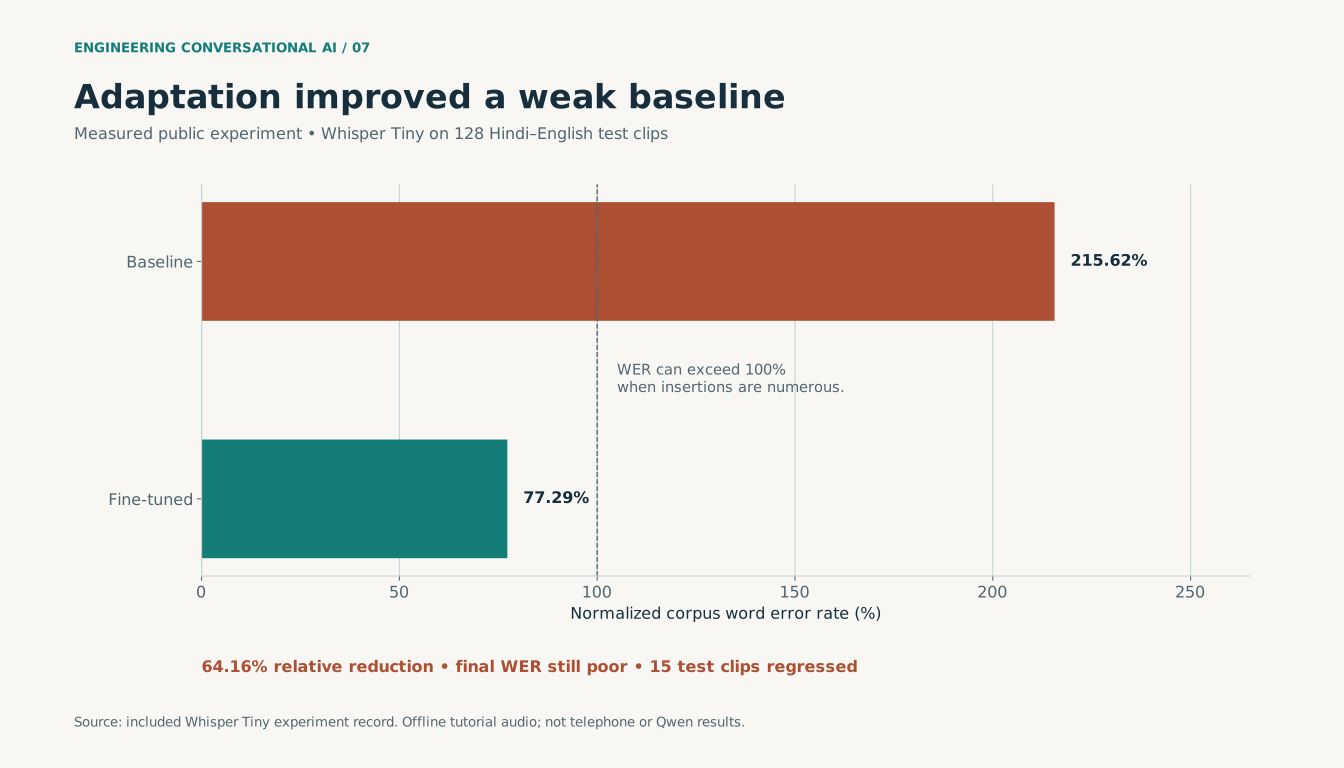
The relative WER reduction was 64.16%, but the final WER remained poor. The fixed Hindi-prompt, greedy-decoding baseline produced substantial repetition and script mismatch. This is evidence that the adaptation pipeline worked, not that it produced a deployment-ready recognizer or beat modern services.
The model was fully fine-tuned for three epochs using FP32, microbatch four, accumulation two and AdamW at 3e-5. Epoch two was selected on validation WER. Validation worsened in epoch three despite lower training loss.
One actual test reference was “एक निमंत्रण पत्र type करें”. The baseline repeated “dal” to its generation limit. The adapted model produced “पर टाइप करें”: much less repetition, but still missing meaningful content. On another clip, a mostly intelligible baseline degraded into repeated phrases after adaptation. Aggregate improvement does not erase those regressions.
The timing experiment used cached features and batch-one offline generation. It excluded audio preprocessing, endpoint detection, transport, the LLM and TTS. Median generation became slower while the tail improved, partly because pathological long outputs decreased. It establishes neither live streaming latency nor concurrent-call capacity.
The measured record and machine-readable comparison preserve the evidence.
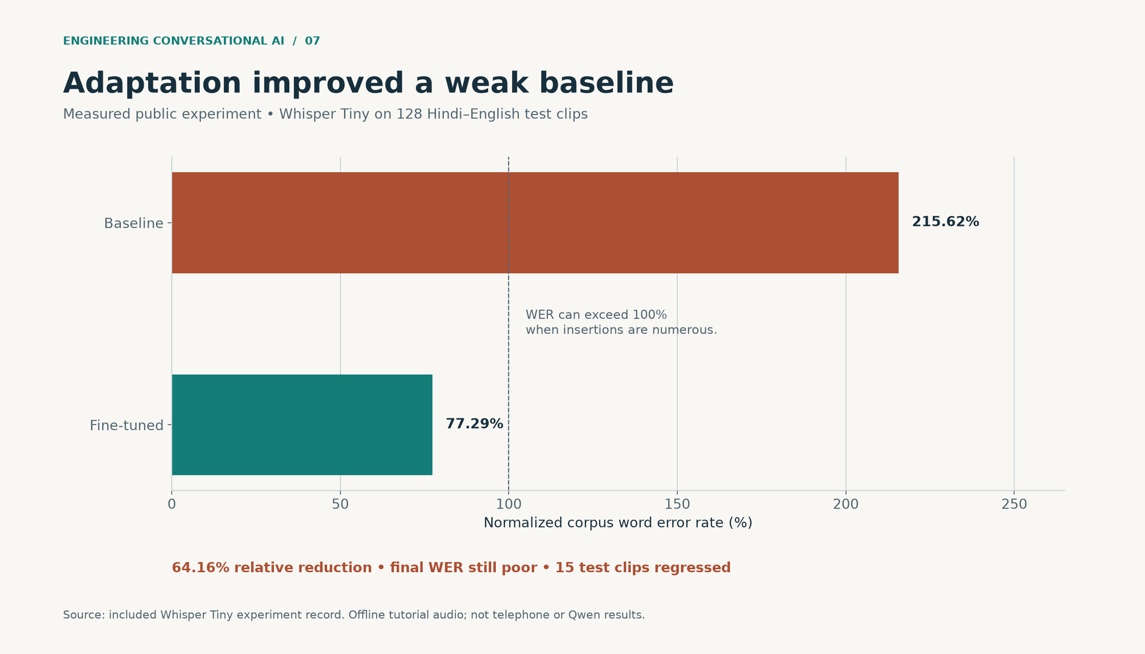
Figure 7. Measured experiment. Measured Whisper Tiny normalized WER fell from 215.62 to 77.29 percent on 128 public test clips; final quality remained poor and 15 clips regressed. Scalable SVG.
The release decision for the new model
The proposed Qwen run should report base and adapted WER, entity accuracy, script-sensitive and secondary normalized scores, p50/p95 finalization delay, hardware memory and live serving capacity. Record the Qwen results under a separate run ID when you execute that comparison.
A defensible first gate is improvement on the target slices without material regression on ordinary English and Hindi, followed by end-to-end tests at 10, 20, 40 and 100 calls. Passing 40 calls does not require claiming 100; a maximum test point can fail and still be useful.
That record is what turns “we fine-tuned a speech model” into a technical story that another engineer can inspect.
The data review that should happen before the first GPU hour
A speech dataset is a collection of recording decisions. Those decisions can explain more of the result than the learning rate.
Consider three constructed annotation examples:
| Heard speech | Primary transcript | Annotation decision |
|---|---|---|
| “Can call me after six, lah.” | Can call me after six lah | Preserve the local expression; omit punctuation only under the declared normalization |
| “मेरा EMI debit नहीं हुआ।” | मेरा EMI debit नहीं हुआ | Preserve the English abbreviation and Hindi negation |
| “Tuesday… sorry, Thursday.” | Tuesday sorry Thursday | Keep the repair; downstream interpretation selects Thursday |
Training the recognizer on “Thursday” alone in the last example teaches a different task: rewriting speech into an interpreted answer. For this system, recognition should preserve enough information to audit the repair.
The manifest audit should reject missing files, invalid duration, empty transcripts for labeled speech and speaker overlap across splits. It should flag clipping, long silence, inconsistent script and unusually high transcript characters per second for human review. A high ratio is a warning, not proof that a fast speaker was mislabeled.
The following small check catches exact source-group leakage. It does not detect acoustic near-duplicates or mislabeled speakers:
def audit_split_groups(rows):
    seen = {}
    for row in rows:
        split = row["split"]
        if split not in {"train", "dev", "test"}:
            raise ValueError("Unknown split")
        for field in ("speaker_group", "source_group"):
            value = row[field]
            if not value:
                raise ValueError(f"Missing {field}")
            key = (field, value)
            previous = seen.setdefault(key, split)
            if previous != split:
                raise ValueError(f"Leaked group: {key}")
    return len(rows)
The source_group identifies the original recording before segmentation. Run this on the rich manifest before exporting trainer-specific JSONL. A random clip split can put adjacent segments of the same tutorial in both training and test. The resulting score measures familiarity with that recording as well as recognition ability.
Know which tokens receive loss
For a token-generating recognizer, the supervised objective is typically a sum of next-token cross-entropies over the designated target tokens:
loss = − sum(mask[t] × log P(target[t] | audio, prefix, earlier targets))
       / sum(mask[t])
The exact prefix, language markers, end tokens and masking rules belong to the selected trainer. Padding must not become an artificial training target. PyTorch cross-entropy supports an ignored target index, commonly −100; this mechanism alone does not decide which model-specific prefix tokens should be masked. Inspect an actual collated batch and decoded labels before starting the run. PyTorch cross-entropy reference.
With a nominal effective batch of sixteen, sixteen very short clips and sixteen long clips do not carry the same acoustic or token workload. Track audio seconds and unmasked target tokens per update alongside examples per update. Bucket by duration to reduce padding, but shuffle within the training policy so one language or recording session does not dominate a long sequence of updates.
For the proposed balanced 40-hour collection, log the sampled language proportions after filtering and resampling. Ten hours on disk per slice does not guarantee equal exposure if one slice contains much shorter utterances.
Separate adaptation from decoding and runtime changes
A useful first ablation has four configurations:
| Configuration | Weights | Decoding | Audio path | Question answered |
|---|---|---|---|---|
| A | Base | Frozen baseline | Original audio | Starting recognition quality |
| B | Base | Tuned on development data | Original audio | Gain from decoding alone |
| C | Adapted | Same as B | Original audio | Added value of weight adaptation |
| D | Same as C | Same as C | Telephone codec round-trip | Sensitivity to the deployment channel |
Measure serving changes in another comparison with the same model and inputs. Changing weights, beam settings, quantization and endpoint thresholds together creates a result that is difficult to explain.
Ordinary English and Hindi are regression slices, even if the business problem is Hinglish or Singlish. Improvement on one distribution can be purchased by forgetting another. In the completed Tiny experiment, 104 test clips improved, 15 regressed and nine were unchanged under the recorded comparison. The regressed examples belong in the report.
A streaming test must not see the future
Offline decoding can inspect the complete utterance. A live recognizer at 900 ms cannot inspect a correction spoken at 1,600 ms.
Replay recorded audio according to its timestamps, exposing only the prefix available at each update. Record the provisional hypothesis, committed prefix, revision count and finalization delay. Then test the same clip with the full offline decoder. The difference is informative; presenting offline WER as a streaming result is not.
For each critical term, keep both first-correct time and stable-correct time. “First correct” is insufficient if the hypothesis later changes to the wrong policy number. The release package should preserve the timeline alongside the final transcript.