Part 17 of 18 · 7 min read
Latency, concurrency and the cost of a completed task
Critical-path analysis, nested limits, cache-aware accounting and load tests that reflect real agent behaviour.
Arunank Sharan · Kuzushi Labs ·
In this article
A fast first token can hide a slow task. A cheap model can become expensive when it repeats tools or needs several repair passes. A service can accept many HTTP requests while only a small number of model streams make progress.
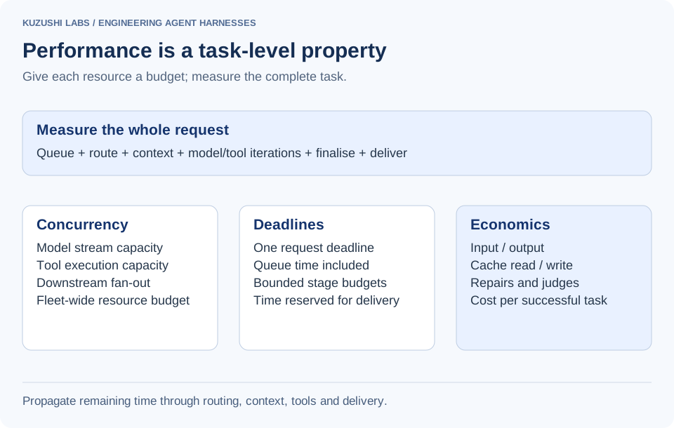
Performance work on an agentic harness needs to measure the complete path: admission, routing, context, model turns, tools, repairs, finalisation and delivery. The client runtime exposes several of these boundaries explicitly, which makes optimisation more precise.
Start with the critical path
For a turn with multiple model iterations, a useful decomposition is:
Total = admission wait + routing + context build
      + Σ(model request + tool batch + repair overhead)
      + finalisation + delivery
Independent hydration calls can overlap. Dependent tool calls cannot. Parallel tool latency is closer to the slowest required call plus scheduling overhead, while sequential tool latency accumulates.
Measure both time to first useful output and time to completed task. A status message saying “checking” can improve perceived responsiveness but does not reduce the time until a guest receives a verified answer.
Control resources independently
Admission, model streams, tool execution and domain fan-out consume different resources. Each needs an explicit concurrency limit, a queue policy and a cancellation rule. Set limits from provider quotas and measured dependency capacity, then validate them with the expected traffic mix.
A semaphore size is not a platform throughput result. Capacity depends on model duration, iteration count, provider quotas, backend latency, replicas and traffic mix. Report measurements with the workload and deployment shape so the reader can interpret what was actually tested.
For a synthetic capacity example, take three worker replicas, a limit of four concurrent composite tools per worker, and a maximum fan-out of six reads per composite tool. The upper bound is 3 × 4 × 6 = 72 simultaneous downstream reads. If the dependency can safely serve only 24, independently tuning each worker is insufficient: use a shared budget or partition the allowance across replicas.
Account for the caller’s deadline
Consider an illustrative caller deadline of 30 seconds. A budget of 4 seconds for routing, 3 for context, 20 for execution and 3 for finalisation and transfer fits within that envelope. These are example allocations for the calculation, not the client’s deployment settings.
If routing consumes 7 seconds and context consumes 4, retaining the full 20-second execution budget leaves too little time to return the result. The execution stage has at most 16 seconds after reserving 3 for finalisation. A component can stay within its own timeout while the end-to-end request still misses the caller’s deadline.
Propagate an absolute request deadline and allocate remaining time at each stage:
def remaining_budget(deadline, now, reserve=0.5):
    return max(0.0, deadline - now - reserve)

assert remaining_budget(30.0, 11.0) == 18.5
The reserve is an illustrative allowance for finalisation and response transfer. In production, compare against a monotonic deadline and pass each stage the smaller of its own limit and the remaining request budget. Include semaphore wait and retries in that accounting. If no useful budget remains, return the defined timeout outcome instead of starting work whose result cannot arrive in time.
Understand nested concurrency limits
A single model turn can request several tools, and one composite booking tool can fan out to several calendars. Limits at these layers govern different resources.
Raising the outer tool limit can multiply inner calendar traffic. Adding replicas multiplies process-local semaphores again. Provider limits and domain-service connection pools are shared constraints, so per-process limits need a deployment-level capacity plan.
An illustrative steady-state calculation uses Little’s Law: average in-flight work equals arrival rate times average time in the system. At two requests per second and eight seconds per request, average in-flight work is sixteen requests. That does not imply sixteen simultaneous provider calls, because requests spend time in other stages, but it gives a first consistency check for admission capacity.
At saturation, queueing dominates. Report queue age and rejected/admitted work, not only handler duration for requests that eventually reached execution.
Price the token classes correctly
Track ordinary input, output, cache-read and cache-creation tokens with model-specific rates. An unknown price should produce an explicit unpriced state. Resolve exact model revisions or deliberate aliases before applying a rate; a similar model name is not sufficient evidence of identical pricing.
Provider usage conventions differ. Some fields include cached input inside total input, while others report disjoint classes. Normalize usage before applying rates, or cache reads can be counted twice.
Using illustrative rates of $1 per million ordinary input tokens, $5 per million output tokens, $0.10 per million cached-read tokens and $1.25 per million cache-write tokens:
| Scenario | Input composition | Output | Cost |
|---|---|---|---|
| No cache | 9,000 ordinary input | 400 | $0.0110 |
| Warm prefix | 1,000 ordinary + 8,000 cache read | 400 | $0.0038 |
| New cache prefix | 1,000 ordinary + 8,000 cache write | 400 | $0.0130 |
The warm-cache saving is about 65.5% for this complete example, not 90% of the whole request. The output cost remains, and creating the cache costs more than an ordinary read under these assumed rates. These are worked arithmetic using an example rate table, not a current provider quote or a client saving claim.
from decimal import Decimal

def cost_usd(tokens, rates_per_million):
    return sum(
        Decimal(tokens.get(kind, 0)) * Decimal(str(rate))
        for kind, rate in rates_per_million.items()
    ) / Decimal(1_000_000)

assert cost_usd(
    {"input": 1000, "output": 400, "cache_read": 8000},
    {"input": 1, "output": 5, "cache_read": 0.1},
) == Decimal("0.0038")
Count the work around the main model
Classification, judges, repair calls, failed requests, retrieval and workflow execution all contribute to cost. The client console separates agent and judge spend, while the model gateway supplies another accounting view.
LiteLLM virtual keys support model access controls, attribution and budgets at the gateway. Those controls apply to traffic that actually goes through the configured gateway path. A direct-provider fallback needs separate visibility and policy. LiteLLM virtual keys
For pricing a product, the useful denominator is a completed task. If a cheaper model reduces per-call cost but doubles unresolved cases, the cost per successful task can worsen. Include human review and escalation workload when comparing operating models.
Optimise by failure mechanism
If context dominates, parallelise independent reads and remove redundant evidence. If the model loops unnecessarily, improve tool contracts or move mandatory sequences into a composite flow. If routing dominates, examine when the classifier calls a model. If output dominates, constrain unnecessary verbosity while preserving the useful answer.
Prompt caching helps repeated stable prefixes. It does not fix slow backend APIs. More replicas help admission capacity. They do not remove a provider quota. A larger model can reduce some reasoning failures, but cannot correct an endpoint that ignores a parameter.
Load-test a realistic mix
Use a workload containing FAQs, booking searches, issue reports, host analysis, duplicates and degraded dependencies. Record latency percentiles, throughput, iteration counts, tool fan-out, queue wait, error rates and cost by scenario class.
Run warm-cache and cold-cache cases separately. Test bursts as well as steady load. Include a slow domain service and provider rate limiting. Confirm that the service remains within its resource limits and produces honest failure outcomes instead of continuing work whose response will be discarded.
Performance is successful when the task finishes correctly within a useful time and cost envelope. The harness makes those dimensions visible enough to improve together rather than optimising one misleading number.