Choosing embeddings for financial evidence

An embedding model is useful when it brings the right evidence into the candidate set. A model with a financial name does not automatically recognise the difference between consolidated and segment revenue, or between an annual figure and a year-to-date figure. Those distinctions still need source structure and metadata.

The client’s dense-embedding adapter used philschmid/bge-base-financial-matryoshka, with a 768-dimensional vector and a CPU execution path. The codebase also contained alternative embedding adapters. The active dense path is the useful starting point for understanding the system, rather than treating every available adapter as a deployed configuration.

What a financial embedding can contribute

The BGE financial model is a fine-tuned sentence-transformer based on BGE base English. Its model card documents a 512-token input limit and Matryoshka training at several dimensions. Those properties affect chunking, storage and the experiments that are possible. Financial BGE model card

The model can help align wording such as “cash generated from operations” with “operating cash flow.” It cannot enforce an issuer filter, validate a unit or guarantee that a cited number is correct. The retrieval contract should keep those responsibilities separate.

For an embedding comparison, use real task shapes: exact financial facts, management explanations, cross-period comparisons and ambiguous terminology. A broad semantic benchmark is useful background, but the release decision should depend on the analyst’s questions.

A million documents is not a million vectors

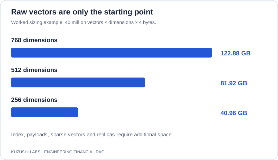
Let D be document count and m the mean number of chunks. The vector count is N = D × m. If a worked example uses one million documents and forty chunks per document, the index contains forty million vectors.

For float32 dense vectors, raw vector storage is:

raw bytes = vector count × dimensions × 4
40,000,000 × 768 × 4 = 122,880,000,000 bytes
                       ≈ 122.88 GB, or 114.44 GiB

This excludes the graph index, payloads, sparse vectors, replicas, write-ahead logs and temporary migration capacity. It is a lower bound, not a server-sizing recommendation.

At 256 dimensions, the corresponding raw vector data would be 40.96 GB. Whether that reduction is useful depends on quality, representation support and the database’s storage configuration.

Matryoshka dimensions are an experiment

Matryoshka training aims to make prefixes of a vector useful at different dimensionalities. That permits a storage–quality comparison without treating arbitrary truncation of every embedding model as valid.

For a supported model, truncate both query and document vectors to the same dimension and renormalise before cosine similarity. Create a distinct index configuration for each dimension. Do not mix 768-dimensional and 256-dimensional vectors under one named-vector contract.

from math import sqrt

def prefix_normalise(vector: list[float], dimensions: int) -> list[float]:
    if not 0 < dimensions <= len(vector):
        raise ValueError("Invalid dimension")
    prefix = vector[:dimensions]
    norm = sqrt(sum(value * value for value in prefix))
    if norm == 0:
        raise ValueError("Zero vector")
    return [value / norm for value in prefix]

The test should compare evidence recall, ranking quality, index size and latency. A small average decline may conceal a large regression on rare financial terminology, so preserve slice-level results.

Dense and sparse representations do different work

The client’s retrieval design also included SPLADE, using naver/splade-cocondenser-ensembledistil. SPLADE produces sparse vocabulary-weighted representations through a language-model-based expansion mechanism. It differs from simply counting keywords and should not be described interchangeably with BM25. SPLADE paper

A sparse representation can help match an exact financial term. Learned expansion can also associate related terms, which is useful but means it is not a strict exact-match filter. Issuer, date and document-type restrictions still belong in metadata constraints.

The important implementation detail is pooling across input positions. Transformer logits have a token-position axis and a vocabulary axis. The stored sparse indexes must identify vocabulary terms, not token positions.

# logits: [batch, sequence_length, vocabulary_size]
# attention_mask: [batch, sequence_length]
weights = torch.log1p(torch.relu(logits))
weights = weights * attention_mask.unsqueeze(-1)
pooled = weights.max(dim=1).values
indices = torch.nonzero(pooled[0] > 0.0, as_tuple=True)[0]
values = pooled[0, indices]

This is the core aggregation shape. In a service, run inference without gradient tracking, batch inputs, pin the tokenizer/model revision and apply a tested sparsity policy. Aggressive pruning can reduce storage while removing the vocabulary terms that helped recall.

Keep the index contract explicit

A passage needs a stable ID and all its representations attached to the same point. A dense+sparse design only works when both vectors are actually persisted and queried under the intended names.

{
  "point_id": "immutable-passage-uuid",
  "vector_names": ["dense", "sparse"],
  "payload": {
    "passage_id": "immutable-passage-uuid",
    "document_version": "example-2024-v1",
    "text": "Source passage with its financial context",
    "issuer_id": "example-co",
    "document_type": "10-K",
    "chunker_version": "filing-blocks-v3",
    "embedding_version": "financial-bge-768-v1"
  }
}

Do not restart point IDs at zero for each document. Do not silently pair the first embedding with the second chunk after filtering empty text. Keep a typed passage record through batching and verify counts and IDs before writing.

These checks are inexpensive and protect against failures that no retrieval benchmark can diagnose if the underlying records have already been misaligned.

Batch offline work; protect interactive work

Document embedding is throughput-oriented. Query embedding is latency-oriented. A CPU path is convenient for an initial implementation, but encoding chunks individually leaves batching opportunities unused.

For offline work, batch similar token lengths, cap total tokens per batch, and measure documents or tokens per second alongside memory. For interactive queries, keep the model warm and avoid waiting behind a long ingestion batch. A separate service or reserved queue provides a clear boundary.

GPU deployment is justified by measured utilisation and cost per encoded token, not by the assumption that every embedding service needs a GPU. A small query workload may be well served on CPU; a corpus-wide migration has a different demand profile.

A modern comparison set

For a new evaluation in 2026, retain the historical financial BGE configuration as a baseline and compare it with a current small embedding model such as Qwen3-Embedding-0.6B, using the query formatting and input contract specified in its model card. Its instruction support creates another experiment: whether task-specific query instructions improve financial evidence retrieval. Qwen3 embedding model card

Do not switch because the newer model has a stronger headline benchmark. Measure the gain against re-embedding cost, larger or smaller vectors, hardware requirements and migration risk.

A safe migration creates a second versioned index, runs shadow queries, checks citation identity and switches an alias only after acceptance. Keep a rollback path and budget temporary dual storage. Improving the retriever should not make old source links disappear.