Part 8 of 12 · 7 min read
On-premises serving: memory, latency and capacity
Weight and KV-cache calculations, a practical local deployment topology, workload matrices and reproducible latency measurements.
Arunank Sharan · Kuzushi Labs ·
In this article
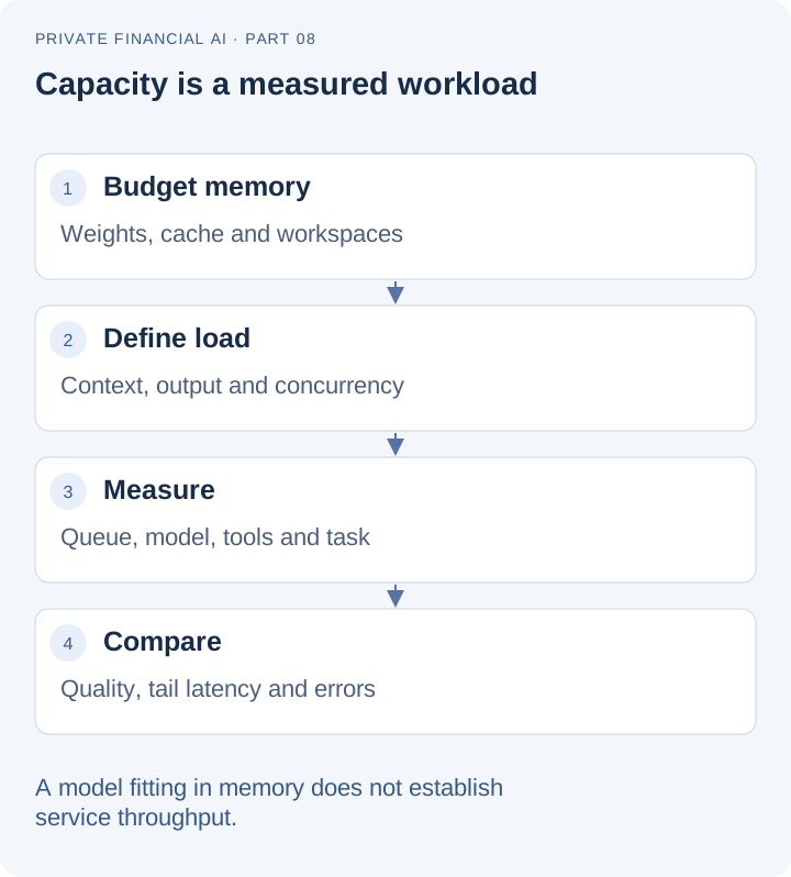
A model that fits on a workstation is not yet a service with a known capacity. Capacity depends on the resident weights, the context kept for each active request, prefill work, generation length, batching and the rest of the application sharing the machine.
For this financial workflow, the useful measurement is time to a correct, reviewable result. Token generation speed contributes to that number, but retrieval, queueing, tool calls and repeated model turns contribute too. This chapter turns those dependencies into a capacity budget and a repeatable measurement procedure.
Count resident parameters, not only the model name
The Gemma 4 model card lists E4B as 4.5 billion effective parameters and 8 billion with embeddings. That distinction matters when estimating storage. A name suggesting “4B” is not a reliable substitute for the actual artifact and runtime allocation.
Here is the elementary weight-only calculation for 8 billion parameters, assuming every parameter used the same storage width:
| Representation | Calculation | Idealized weight storage |
|---|---|---|
| BF16 | 8 billion × 2 bytes | 16 GB / 14.90 GiB |
| INT8 | 8 billion × 1 byte | 8 GB / 7.45 GiB |
| 4-bit | 8 billion × 0.5 bytes | 4 GB / 3.73 GiB |
These are arithmetic lower-level estimates, not measured residency. Quantization metadata, unquantized tensors, adapters, modality components, runtime workspaces and allocator overhead add memory. Some engines offload particular tables or components. Inspect the exported artifact and measure the process rather than treating this table as a GPU purchase recommendation.
A 24 GiB GPU is a concrete evaluation candidate for the reference recipe, not a certified capacity claim. Whether the training or serving configuration fits depends on sequence length, modules loaded, batch size and kernel support. Establish fit with a short representative run before expanding the workload.
Add the key-value cache
For a conventional decoder with full attention, a useful simplified KV estimate is:
bytes = 2 × layers × KV_heads × head_dimension × tokens × bytes_per_element × active_sequences
The factor of two accounts for keys and values. For an illustrative architecture with 32 layers, 8 KV heads, head dimension 128, 8,192 cached tokens and two-byte cache values, one sequence needs 1 GiB of KV storage. Eight such sequences need 8 GiB before other allocations.
def dense_kv_bytes(layers, kv_heads, head_dim, tokens, sequences, dtype_bytes=2):
    return 2 * layers * kv_heads * head_dim * tokens * sequences * dtype_bytes

assert dense_kv_bytes(32, 8, 128, 8192, 1) == 1024 ** 3
This example is not Gemma 4’s exact cache formula. Hybrid local/global attention, sliding windows, cache quantization and engine-specific storage change the calculation. Use the model configuration to estimate each layer type separately, then compare with observed allocation at the intended request lengths.
The PagedAttention paper explains how managing KV memory in blocks can improve serving efficiency. It does not remove the need to budget the live context or guarantee that a particular model/runtime combination supports the same optimizations.
Keep the deployment topology straightforward
A private service has an authenticated gateway, an orchestration process, local inference, permissioned retrieval or portfolio services, deterministic tools and a restricted observability path. Place the inference endpoint on a private interface. The browser talks to the application gateway, not directly to an unrestricted model server.
The model artifact is imported through an approved update path. The runtime starts with local files. Public dataset acquisition and model downloads happen in the separate preparation environment. Record digests before import and verify them again inside the restricted environment.
The reference benchmark adapter connects only to a loopback Ollama /api/chat endpoint, disables proxy use and rejects redirects. That makes its network behaviour simple to inspect. The Ollama chat API documentation describes the request shape used by the adapter.
{
  "model": "your-local-candidate",
  "stream": false,
  "format": "json",
  "options": {"temperature": 0, "num_predict": 512},
  "keep_alive": "5m",
  "messages": [
    {"role": "system", "content": "Return a bounded financial decision."},
    {"role": "user", "content": "Project INR 25 lakh for five years at 6%."}
  ]
}
The model name above is a locally installed candidate identifier. Loading or exporting a model into that runtime is a separate compatibility step. The runner’s JSON protocol is application-level structured output, not a claim that every model supports a provider’s native function-calling format.
Measure the latency components separately
For an agent request, total time includes admission queueing, prompt preparation, model prefill, decoding, tools and result assembly. A two-tool task can include three model decisions. Measuring only the final decode hides much of the user’s wait.
Instrument monotonic timestamps around each boundary. For streaming interfaces, record time to the first displayed useful content as well as completion time. A partial JSON token is not useful content just because it arrived quickly.
| Measurement | Start and stop | Why it matters |
|---|---|---|
| Queue time | Request admitted → execution begins | Saturation and fairness |
| Model first token | Inference request → first generated token | Prefill and scheduling |
| Model completion | Inference request → final model output | Generation budget |
| Tool latency | Tool admitted → result or timeout | Downstream dependency |
| Task latency | User request → validated final outcome | End-user experience |
| Accepted-task latency | Same boundary, only correctly completed tasks | Quality-adjusted service experience |
Report all-attempt latency alongside accepted-task latency. A fast refusal to every request must not look like a superior service. Include timed-out and failed requests in the attempted count and report their rate explicitly.
Use a workload matrix instead of one impressive prompt
A useful initial load matrix crosses four input lengths with four active-request counts: 512, 2,048, 4,096 and 8,192 tokens; concurrency 1, 2, 4 and 8. That creates 16 workload cells. Repeat with a 128-token and a 512-token output cap when longer explanations are part of the product.
Keep the task mix fixed within a comparison: calculations, snapshot summaries, clarifications and unavailable-tool cases. Separate cold model load from warm inference. State whether retrieval and tool fixtures are local or live, and whether the queueing model is closed-loop concurrency or an externally paced arrival rate.
At each cell, record attempted requests, successful contracts, wall-clock duration, p50/p95/p99 task latency, output tokens, peak GPU memory and errors. Hold a workload long enough to expose steady-state behaviour rather than reporting only the first few requests.
Do not infer concurrent capacity from the kit’s serial runner. It is designed for inspectable functional comparisons. A service-load experiment needs a separate concurrent driver and measured admission behaviour.
Summarize collected timings without inventing precision
The kit includes a latency summarizer for candidate JSONL files. It uses nearest-rank percentiles and reports the number of timed attempts.
import math

def nearest_rank(values, fraction):
    if not values:
        return None
    ordered = sorted(values)
    index = max(0, math.ceil(fraction * len(ordered)) - 1)
    return ordered[index]

assert nearest_rank([100, 120, 150, 200, 900], 0.95) == 900
With 24 cases, p95 is effectively a tail observation in a very small sample. Report the sample size and retain individual timings. For production capacity, collect repeated measurements under a specified load and summarize across runs as well as requests.
python summarise_latency.py /tmp/candidate-predictions.jsonl
No service latency or throughput value is supplied in place of a measurement. The reference kit produces the fields needed to collect and report those values on the chosen hardware.
Optimize the bottleneck that the trace identifies
If queueing dominates, adding a longer prompt or enabling more reasoning will make the problem worse. If prefill dominates, shorten irrelevant evidence and inspect prefix-cache behaviour. If tool latency dominates, improve the data service or reduce redundant reads. If decoding dominates, shorten the structured result and avoid asking the model to restate the entire source document.
Continuous batching can improve aggregate throughput while changing individual-request latency. A larger batch is not automatically a better user experience. Reserve capacity for bounded interactive requests or apply admission limits when long analytical work shares the same model server.
Finally, keep the release rollback operationally simple. Retain the previous model, adapter, template and runtime configuration as a named bundle. A capacity regression should be reversible without rebuilding the data pipeline. The release procedure in Part 12 ties those artifacts to the quality and latency report.